function [J, grad] = linearRegCostFunction(X, y, theta, lambda) %LINEARREGCOSTFUNCTION Compute cost and gradient for regularized linear %regression with multiple variables % [J, grad] = LINEARREGCOSTFUNCTION(X, y, theta, lambda) computes the % cost of using theta as the parameter for linear regression to fit the % data points in X and y. Returns the cost in J and the gradient in grad
% Initialize some useful values m = length(y); % number of training examples
% You need to return the following variables correctly J = 0; grad = zeros(size(theta));
% ====================== YOUR CODE HERE ====================== % Instructions: Compute the cost and gradient of regularized linear % regression for a particular choice of theta. % % You should set J to the cost and grad to the gradient. %
function [error_train, error_val] = ... learningCurve(X, y, Xval, yval, lambda) %LEARNINGCURVE Generates the train and cross validation set errors needed %to plot a learning curve % [error_train, error_val] = ... % LEARNINGCURVE(X, y, Xval, yval, lambda) returns the train and % cross validation set errors for a learning curve. In particular, % it returns two vectors of the same length - error_train and % error_val. Then, error_train(i) contains the training error for % i examples (and similarly for error_val(i)). % % In this function, you will compute the train and test errors for % dataset sizes from 1 up to m. In practice, when working with larger % datasets, you might want to do this in larger intervals. %
% Number of training examples m = size(X, 1);
% You need to return these values correctly error_train = zeros(m, 1); error_val = zeros(m, 1);
% ====================== YOUR CODE HERE ====================== % Instructions: Fill in this function to return training errors in % error_train and the cross validation errors in error_val. % i.e., error_train(i) and % error_val(i) should give you the errors % obtained after training on i examples. % % Note: You should evaluate the training error on the first i training % examples (i.e., X(1:i, :) and y(1:i)). % % For the cross-validation error, you should instead evaluate on % the _entire_ cross validation set (Xval and yval). % % Note: If you are using your cost function (linearRegCostFunction) % to compute the training and cross validation error, you should % call the function with the lambda argument set to 0. % Do note that you will still need to use lambda when running % the training to obtain the theta parameters. % % Hint: You can loop over the examples with the following: % % for i = 1:m % % Compute train/cross validation errors using training examples % % X(1:i, :) and y(1:i), storing the result in % % error_train(i) and error_val(i) % .... % % end %
function [X_poly] = polyFeatures(X, p)
%POLYFEATURES Maps X (1D vector) into the p-th power
%   [X_poly] = POLYFEATURES(X, p) takes a data matrix X (size m x 1) and
%   maps each example into its polynomial features where
%   X_poly(i, :) = [X(i) X(i).^2 X(i).^3 ...  X(i).^p];
%


% You need to return the following variables correctly.
X_poly = zeros(numel(X), p);

% ====================== YOUR CODE HERE ======================
% Instructions: Given a vector X, return a matrix X_poly where the p-th
%               column of X contains the values of X to the p-th power.
%
%

for j = 1:p
 X_poly(:,j) = X.^j;
end
% =========================================================================
end
function [lambda_vec, error_train, error_val] = ... validationCurve(X, y, Xval, yval) %VALIDATIONCURVE Generate the train and validation errors needed to %plot a validation curve that we can use to select lambda % [lambda_vec, error_train, error_val] = ... % VALIDATIONCURVE(X, y, Xval, yval) returns the train % and validation errors (in error_train, error_val) % for different values of lambda. You are given the training set (X, % y) and validation set (Xval, yval). %
% Selected values of lambda (you should not change this) lambda_vec = [0 0.001 0.003 0.01 0.03 0.1 0.3 1 3 10]';
% You need to return these variables correctly. error_train = zeros(length(lambda_vec), 1); error_val = zeros(length(lambda_vec), 1);
% ====================== YOUR CODE HERE ====================== % Instructions: Fill in this function to return training errors in % error_train and the validation errors in error_val. The % vector lambda_vec contains the different lambda parameters % to use for each calculation of the errors, i.e, % error_train(i), and error_val(i) should give % you the errors obtained after training with % lambda = lambda_vec(i) % % Note: You can loop over lambda_vec with the following: % % for i = 1:length(lambda_vec) % lambda = lambda_vec(i); % % Compute train / val errors when training linear % % regression with regularization parameter lambda % % You should store the result in error_train(i) % % and error_val(i) % .... % % end % %
for i=1:size(lambda_vec, 1) theta = trainLinearReg(X, y, lambda_vec(i)); error_train(i) = linearRegCostFunction(X, y, theta, 0); error_val(i) = linearRegCostFunction(Xval, yval, theta, 0); end
Once we have done some trouble shooting for errors in our predictions by:
1.Getting more training examples 2.Trying smaller sets of features 3.Trying additional features 4.Trying polynomial features 5.Increasing or decreasing λ 6.We can move on to evaluate our new hypothesis.
A hypothesis may have a low error for the training examples but still be inaccurate (because of overfitting). Thus, to evaluate a hypothesis, given a dataset of training examples, we can split up the data into two sets: a training set and a test set. Typically, the training set consists of 70 % of your data and the test set is the remaining 30 %.
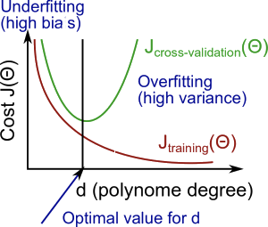
Diagnosing Bias vs. Variance
High bias (underfitting): both $J_{train}(\Theta)$ and $J_{CV}(\Theta)$ will be high. Also, $J_{CV}(\Theta) \approx J_{train}(\Theta)$ High variance (overfitting): $J_{train}(\Theta)$ will be low and $J_{CV}(\Theta)$ will be much greater than $J_{train}(\Theta)$ The is summarized in the figure below:
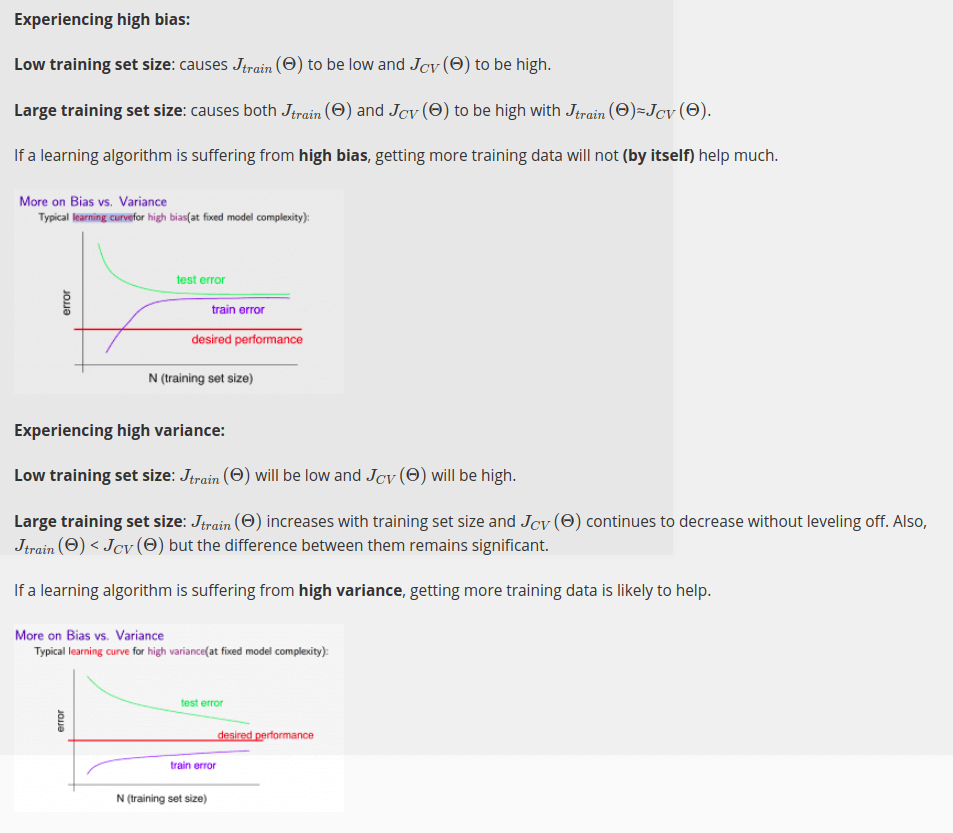
Learning Curves
Deciding What to Do Next Revisited
Our decision process can be broken down as follows:
Getting more training examples: Fixes high variance
Trying smaller sets of features: Fixes high variance