《机器学习实战》第五章(Logistic回归)代码实现以及讲解

Preface

本文是对《机器学习实战》第五章Logistic回归的实践以及一些细节的讲解记录.

完整代码以及数据集见github

---

概述

$$图(1)$$

---

这里我要先讲一点东西,为后面开始做铺垫

对于线性模型的函数,有如下的式子

$f(x) = w_1 x_1 + w_2 x_2 + … + w_n x_n + b$

用向量形式写成

$f(x) = w^T + b$

---

下面这是Logistic回归的假设函数

$h\theta(x) = g(\theta^T * x)$
$g(z) = \frac{1}{1+e^-z}$

这里的g就是sigmoid函数,如果把sigmoid的函数输入记为z,可以有如下式子

$z = w_0 x_0 + w_1 x_1 + w_2 x_2 + … + w_n x_n$

向量形式就是　$z = w^T$

有些地方也会看到如下式子
$h\theta(x) = g(\theta_0 + \theta_1 x_1 + \theta_2 x_2 + …)$

这里需要注意的是多出来的这个$w_0 x_0$,$theta_0$,其实就是对应的前面的b常数项,然后一个常数项 * $x_0$ (若$x_0$取值为１),值是不会变的。后面的代码会涉及到此。

当然这里都是讨论的都是一次的,都是线性的情况,若是更高次,就可以处理非线性的情况。

---

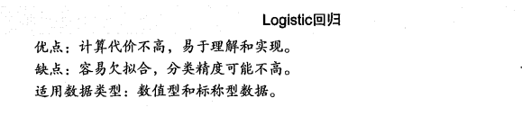
梯度上升(下降)

我们进行训练的目的就是找到最佳回归系数,也就是$ｗ$向量。

这里我们使用梯度上升（下降）法，这里下降与上升只是一个符号(+ or -)的区别，但是本质上都是沿着该函数的梯度方向探寻，这里讲了方向，并未讲到移动量的大小。我们可以称其为步长a。这里步长的选取是有说法的，如果选取太大会导致结果发散；如果选取得太小呢又会使得时间复杂度很高。

停止条件,通常我们可以设置迭代次数，也可以设置一个迭代终止的误差条件。

下面这是梯度下降的公式

$$图(2)$$

---

训练算法: 使用梯度上升找到最佳参数　

伪代码如下
每个回归系数初始化为１
重复Ｒ次
　　　　　计算整个数据集的梯度
　　　　　使用alpha * gradient 更新回归系数的向量
返回回归系数

---

from numpy import *

def loadDataSet():
    dataMat = []
    labelMat = []
    fr = open('testSet.txt')
    for line in fr.readlines():
        lineArr = line.strip().split()
        """
        书上这里说是:为了方便计算,该函数还将X0的值设为1.0
        这里其实是有公式可以参考的,回到线性假设的公式,对应的就是那个常数项
        比如常数项是theta,就可以看做theta * x, x为1.0
        书上说方便,就在于,取1不会改变原来的值
        把这个常数项看做X为1.0,这样在后面就可以通过矩阵来进行计算了 
        """
        dataMat.append([1.0, float(lineArr[0]), float(lineArr[1])])
        labelMat.append(int(lineArr[2]))
    return dataMat, labelMat

def sigmoid(inX):
    return 1.0 / (1 + exp(-inX))


def gradAscent(dataMatIn, classLabels):
    """ 梯度上升求解最佳回归系数

    Args:
        dataMatIn: {List} 样本数据,对应假设中的x
        classLabels: {List} 样本数据,对应假设中的函数值h(x)

    Returns:
        weights: 最佳回归系数矩阵
    """
    dataMatrix = mat(dataMatIn)
    labelMat = mat(classLabels).transpose()
    m,n = shape(dataMatrix)
    # 向目标移动的步长
    alpha = 0.001
    # 迭代次数
    maxCycles = 500
    weights = ones((n,1))
    for k in range(maxCycles):
    #　参考图二公式,这里是梯度上升
        h = sigmoid(dataMatrix * weights)
        error = (labelMat - h)
        weights = weights + alpha * dataMatrix.transpose() * error
    return weights

---

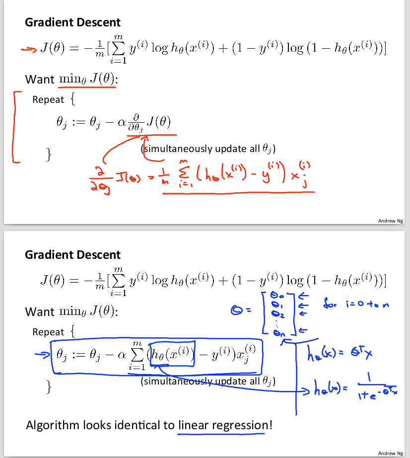
分析数据: 画出决策边界　

def plotBestFit(weights):
    """ 画出数据集和Logistic回归最佳拟合直线的函数

    Args:
        weights: 最佳回归系数矩阵
    """
    import matplotlib.pyplot as plt
    dataMat,labelMat=loadDataSet()
    dataArr = array(dataMat)
    n = shape(dataArr)[0]
    xcord1 = []
    ycord1 = []
    xcord2 = []
    ycord2 = []
    for i in range(n):
        if int(labelMat[i])== 1:
            xcord1.append(dataArr[i,1]); ycord1.append(dataArr[i,2])
        else:
            xcord2.append(dataArr[i,1]); ycord2.append(dataArr[i,2])
    fig = plt.figure()
    ax = fig.add_subplot(111)
    ax.scatter(xcord1, ycord1, s=30, c='red', marker='s')
    ax.scatter(xcord2, ycord2, s=30, c='green')
    x = arange(-3.0, 3.0, 0.1)
    # 最佳拟合直线
    y = (-weights[0]-weights[1]*x)/weights[2]
    ax.plot(x, y)
    plt.xlabel('X1'); plt.ylabel('X2');
    plt.show()

上面注释最佳拟合直线处,设置了sigmoid函数为0。 0是两个分类(类别１和类别0)的分界处。因此我们设定$0 = w_0 x_0 + w_1 x_1 + w_2 x_2$,然后接触X2和X1的关系式(即分割线的方程,X0 =1)

$$图(3) 梯度上升算法在500次迭代后得到的Logistic回归最佳拟合直线$$

---

训练算法: 随机梯度上升　

梯度上升算法在每次更新回归系数时都需要遍历整个数据集,该方法在100个左右的数据集时尚可,但如果有数十亿样本和成千上万的特征,那么该方法的计算复杂度就太高了。

一种改进方式是一次仅用一个样本点来更新回归系数,该方法称为随机梯度上升算法。　由于可以在新样本到来时对分类器进行增量更新,因而随机梯度上升算法是一个在线学习算法。与“在线学习”相对应,一次处理所有数据被称为“批处理”。

随机梯度上升算法伪代码如下

所有回归系数初始化为１
对数据集中每个样本
　　　计算该样本的梯度
使用alpha * gradient更新回归系数
返回回归系数

def stocGradAscent0(dataMatrix, classLabels):
    """ 随机梯度上升算法

        Args:
            dataMatrix:  样本数据,对应假设中的x
            classLabels:  样本数据,对应假设中的函数值h(x)

        Returns:
            weights: 最佳回归系数
    """
    m,n = shape(dataMatrix)
    alpha = 0.01
    weights = ones(n)
    for i in range(m):
        h = sigmoid(sum(dataMatrix[i] * weights))
        error = classLabels[i] - h
        weights = weights + alpha * error * dataMatrix[i]
    return weights

随机梯度上升算法和梯度上升算法很相似,有仍有一些区别,如下:

1. 后者的变量h和误差error都是向量,而前者则全是数值
2. 前者没有矩阵转置过程,所有变量的数据类型都是Numpy数组

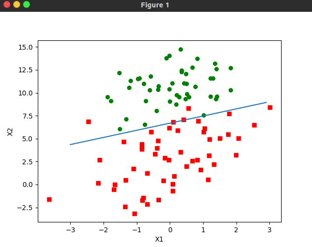
可视化:

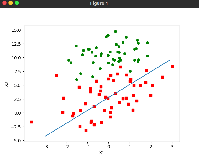
$$图(4)随机梯度上升算法在上述数据集上的执行结果,最佳拟合执行并非最佳分类线$$

图(4)的拟合直线效果还不错,但和图(3)就不那么完美了。当然直接这样比较是有失公允的,后者的结果是在整个数据集上迭代了500次才得到的。

一个判断优化算法优劣的可靠方法是看它是否收敛,也就是说参数是否达到了稳定值,是否还会不断地变化　

---

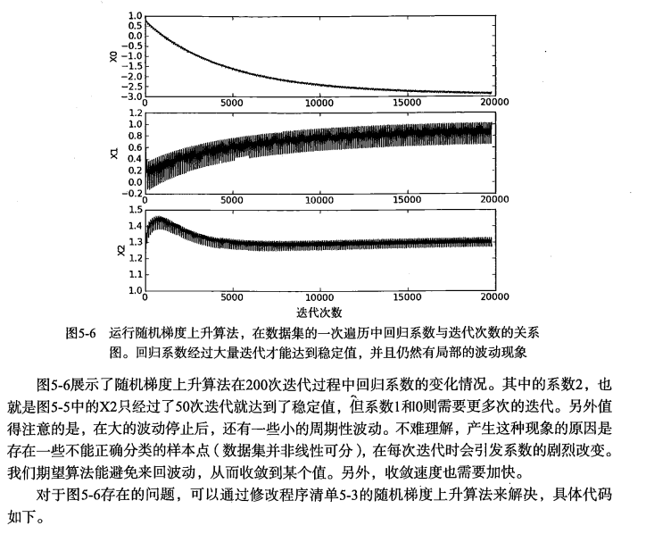
下图是对随机梯度上升算法做了些修改,使其在整个数据集上运行200次。最终绘制的三个回归系数的变化情况

$$图(5)$$

---

改进的随机梯度上升算法　

def stocGradAscent1(dataMatrix, classLabels, numIter=150):
    """ 改进的随机梯度上升算法

        Args:
            dataMatrix:  样本数据,对应假设中的x
            classLabels:  样本数据,对应假设中的函数值h(x)
            numIter: 迭代次数

        Returns:
            weights: 最佳回归系数
    """
    m,n = shape(dataMatrix)
    weights = ones(n)
    for j in range(numIter):
        dataIndex = range(m)
        for i in range(m):
            """
            这是第一处改进地方.alpha在每次迭代时都会调整,这缓解了图(5)上数据波动或者高频波动。
            另外alpha会随着迭代次数不断减小,但永远不会减小到0。    
            必须这样做的原因是为了保证在多次迭代之后新数据仍然具有一定的影响
            如果要处理的问题是动态变化的,可以适当加大上述常数项,来确保新的值获得更大的回归系数
            """
            alpha = 4 / (1.0 + j + i) + 0.01
            """
            这是第二处改进的地方,这里通过随机选取样本来更新回归系数,这种方法将减少周期性波动    
            """ 
            randIndex = int(random.uniform(0, len(dataIndex)))
            h = sigmoid(sum(dataMatrix[randIndex] * weights))
            error = classLabels[randIndex] - h
            weights = weights + alpha * error * dataMatrix[randIndex]
            del(list(dataIndex)[randIndex])
    return weights

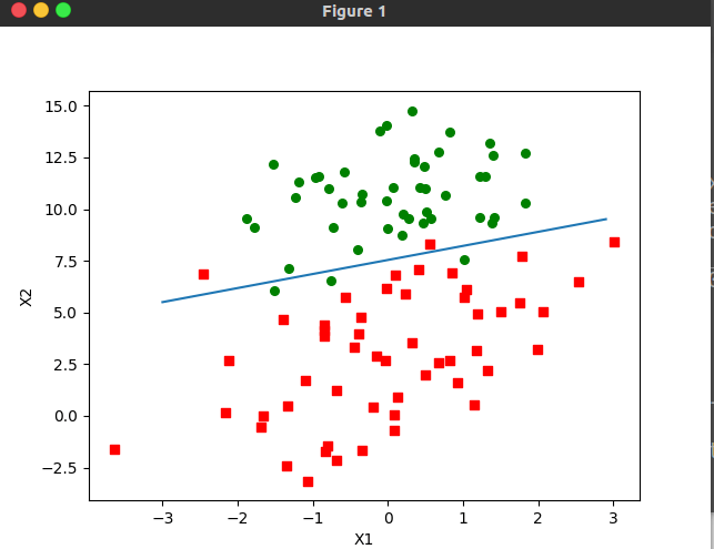
可视化(该分隔线达到了与gradAscent差不多的效果,但是所用的计算量更少):

---

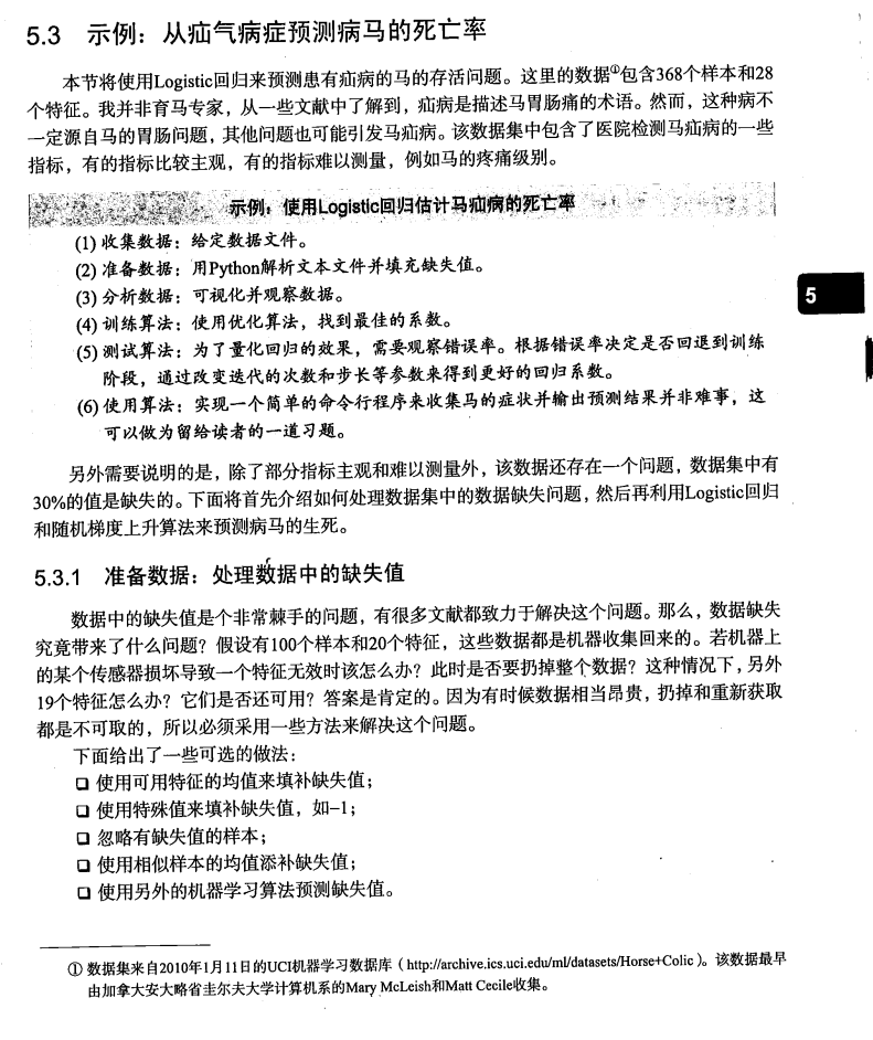
示例: 从疝气病预测病马的死亡率　

原始数据集

def classifyVector(inX, weights):
    """ 分类

        Args:
            inX:  特征向量
            weights: 回归系数

        Returns:
            1 or 0
    """
    prob = sigmoid(sum(inX * weights))
    if prob > 0.5: return 1.0
    else: return 0.0

def colicTest():
    frTrain = open('horseColicTraining.txt')
    frTest = open('horseColicTest.txt')
    trainingSet = []
    trainingLabels = []
    for line in frTrain.readlines():
        currLine = line.strip().split('\t')
        lineArr = []
        for i in range(21):
            lineArr.append(float(currLine[i]))
        trainingSet.append(lineArr)
        trainingLabels.append(float(currLine[21]))
    trainWeights = stocGradAscent1(array(trainingSet), trainingLabels, 500)
    print(trainWeights);
    errorCount = 0
    numTestVec = 0.0
    for line in frTest.readlines():
        numTestVec += 1.0
        currLine = line.strip().split('\t')
        lineArr = []
        for i in range(21):
            lineArr.append(float(currLine[i]))
        if int(classifyVector(array(lineArr), trainWeights)) != int(currLine[21]):
            errorCount += 1
    errorRate = (float(errorCount) / numTestVec)
    print('the error rate of this test is : %f' % errorRate)
    return errorRate

def multiTest():
    numTests = 10
    errorSum = 0
    for k in range(numTests):
        errorSum += colicTest()
    print('after %d iterations the average error rate is : %f ' % (numTests, errorSum / float(numTests)))

the error rate of this test is : 0.298507
the error rate of this test is : 0.402985
the error rate of this test is : 0.358209
the error rate of this test is : 0.432836
the error rate of this test is : 0.283582
the error rate of this test is : 0.313433
the error rate of this test is : 0.522388
the error rate of this test is : 0.283582
the error rate of this test is : 0.283582
the error rate of this test is : 0.253731
after 10 iterations the average error rate is : 0.343284

十次迭代过后的平均错误率为34.33%。事实上,这个结果并不差,因为有30%的数据缺失。

当然如果调整colicTest()中的迭代次数和stocGradAscent1()中的步长,平均错误率可以降到20％左右。

---

总结

---

参考

Markdown中数学公式整理
markdown编辑数学公式
对线性回归、逻辑回归、各种回归的概念学习
机器学习05（logistic回归）
最小二乘法
Logistic回归-小结
matplotlib
Matplotlib中的scatter函数
Matplotlib系列—pyplot的plot( )函数
原[完]Python函数 range()和arange()
从零开始学Python【15】–matplotlib(散点图)
《机器学习实战》5.Logistic回归源码实现
numpy： matrix.getA()
疝气
Horse Colic Data Set